Use harmonic analysis to calculate the peak steady state response due to harmonic loads or base excitations.
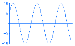
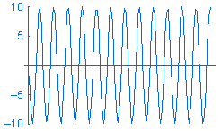
A harmonic load P is expressed as P = A sin (ωt + φ) where: A is the amplitude, ω is the frequency, t is time, and φ is the phase angle. Sample harmonic loads of different frequencies w versus time are shown below:


Although you can create a modal time history study and define loads as functions of time, you may not be interested in the transient variation of the response with time. In such cases, you save time and resources by solving for the steady-state peak response at the desired operational frequency range using harmonic analysis.
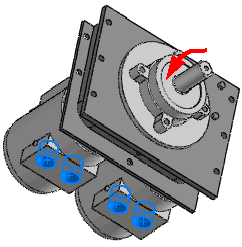
For example, a motor mounted on a test table transfers harmonic loads to the support system through the bolts. You can model the supporting system and define a harmonic study to evaluate the steady-state peak displacements, stresses, etc. for the motor’s range of operating frequencies. You can approximate the motor by a distributed mass.

After running the study, you can view peak amplitudes of response parameters (stresses, displacements, accelerations, and velocities), as well as response graphs of phase angles of response parameters over the range of operating frequencies.
When you run a harmonic study, the contour plot of a response parameter displays the absolute peak values of the response sinusoidal time history at a particular frequency step. The transient sinusoidal part of the response parameter and its phase angle are not shown in the plot. For an operating frequency step that is close to one of the model's natural frequency, the plot of a mode shape is a more realistic representation of the deformed shape than the displacement contour plot at that particular frequency.
You can create a response graph of the phase angle for a response parameter (displacement, stress, velocity, or acceleration) over all solution frequency steps.
Modal, Rayleigh, and Composite modal damping options are available for this type of analysis.