Time Curve
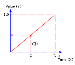
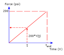
The Time Curve dialog box lets you define or import a time curve to define time-dependent quantities for nonlinear and transient thermal studies. You define X and Y pairs or read them from a text file. The Y value of the time curve is a multiplier to the associated quantity. For example, a force of 200 psi associated with time curve A specifies a force as shown in curve B. At any instant of time (t), the value of the force applied by the program is the specified force magnitude times the Y-value of curve A at time (t). You can define up to 5000 points
|

|

|
|
Curve A - Time Curve
|
Curve B - Actual Force
|
For transient thermal studies, you can specify variation with time for temperature, convection, heat flux, heat power, and radiation. You can define a time curve when specifying the variation of a quantity with time for a particular study or you can save the curve to a library for retrieval by other documents.
To define a time curve:
-
In the PropertyManager of a load or restraint in a transient thermal or nonlinear study, under Variation with time, do one of the following:
-
Click Linear to use the default linear curve of load vs. time. If you select this option, go directly to step 7.
-or-
Click Curve to specify your own variation of load versus time. If you select this option, continue with the next step.
-
In the Time Curve dialog box:
-
In the Curve information box, do the following:
-
-
In the Curve data box, do the following:
-
Set the Units for the X (Time) column.
-
The Y values are dimensionless multipliers to the quantity specified in the PropertyManager for the associated load/restraint.
-
Edit the curve data as desired (Available only when Shape is set to User defined. To get the curve from an external file, click Get curve to open the Function Curves dialog box.
 The X-Y columns show the default values based on the selected shape. You can edit the values in the cells as desired. To add a row, double-click in any cell in the Points column. To delete selected rows, right-click the selection and select Delete.
The program adds the extension .cwcur to the filename. The specified curve can be used in other documents.
-
In the load/fixture PropertyManager, to view the actual values of the specified load/restraint, under Variation with time click View
-
Close the graph window.
 In a nonlinear study, if you do not define a time curve for a load or a restraint, the program uses the default linear time curve.
To use a time curve from an existing library:
-
In a load/fixture PropertyManager of a transient thermal or nonlinear study, under Variation with time, click Curve then click Edit.
-
In the Time curve dialog box, click Get Curve.
-
In the Function Curves dialog box:
-
-
Select the desired curve library file (*.cwcur). The existing curve data files are listed under Time curve.
-
Under Curve Library, select the desired time curve.
The curve data appears in the dialog box.
-
If needed, modify the curve data.
-
Click OK.
-
In the Time Curve dialog box, click OK.