You can use the Underconstrained
Bodies tool to detect any rigid (or free) body modes of bodies that are not
adequately supported by fixtures, connectors, or bonded interaction conditions.
To detect underconstrained bodies, do one of the
following:
- From a static study tree, right-click Connections
 and click Underconstrained Bodies
 .
.
- From the CommandManager, select Diagnostic Tools, and click Underconstrained Bodies
.
- From the dialog box, select Automatically
detect underconstrained bodies.
As a best practice, before you run the Underconstrained Bodies tool, define realistic materials, loads,
and boundary conditions for your model. The study properties should reflect, as
accurately as possible, the operating loads and boundary conditions of the model you
are trying to analyze.
For each part of an assembly, the algorithm checks for free
translations and rotations in the global X, Y, and Z direction and also in oblique
directions. It is also able to detect instability issues in assemblies with chain
(or hinge) mechanisms between parts. In cases where free body modes are detected,
the Underconstrained Bodies tool animates
them accordingly.
The detection of underconstrained bodies is based on the
transformation of the stiffness matrix associated with a finite element model to a
reduced-size stiffness matrix (typically with three translational and three
rotational degrees of freedom per body). The underconstrained modes of the reduced
system are equivalent to the original system of equations.
The transformation of the global stiffness matrix to a reduced-size
stiffness matrix is completed by:
- Introducing a single representative node (reference point)
with six degrees of freedom for each body that represent the translational
and rotational motion of each body
- Transforming the element stiffness matrices by replacing the
original degrees of freedom with the degrees of freedom of the
representative nodes
- Assembling the transformed element stiffness matrices to
determine the reduced-size stiffness matrix
Advantages
The solution is much faster. The performance improvement is based on
the adoption of the Singular Value Decomposition (SVD) technique that is performed
over the reduced stiffness matrix. The reduced stiffnesses are calculated from the
interface surface interaction between bodies originating from boundary conditions,
bonded and contact interactions, or connectors.
The following is an example of a reduced stiffness matrix:
|
|
 |
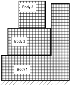
| Each body reduces to one reference point in
the stiffness matrix. The global stiffness matrix reduces from
hundreds of thousands of degrees of freedom to only 18 (3 bodies
x 6 degrees of freedom). |
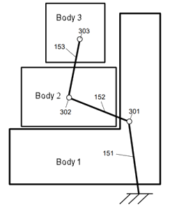
The method considers stiffnesses that
originate from the interactions between bodies. Bodies 1 and 2
come into contact, so the method considers the effect of their
stiffnesses between their reference points. The method considers
stiffnesses that originate from boundary conditions as well, for
example, the stiffness between Body 1 and the ground. |
The SVD technique decomposes the reduced stiffness matrix to three
matrices.
The U and V vectors are orthonormal to each other and describe the
shape of the displacement field. The middle matrix is a diagonal matrix. The
diagonal terms represent the relative stiffnesses of the links between the bodies or
between a body and the ground. If any of the diagonal terms is zero or close to
zero, then this is an indication of a rigid body mode.
You can view animations of the unconstrained displacements of the
whole assembly.
You can view animated translations or rotations in oblique
directions.